
![]()
![]()
![]()
![]()
First NOTCam Science Grade Array (SWIR2)Content of this page:
Detector overview
NOTCam is offered with two possible readout modes: the standard
reset-read-read mode and a ramp-sampling mode
(multiple non-destructive reads during the integration). Read more
about this in NOTCam User's Guide.
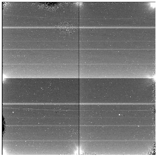
Cosmetics - bad pixels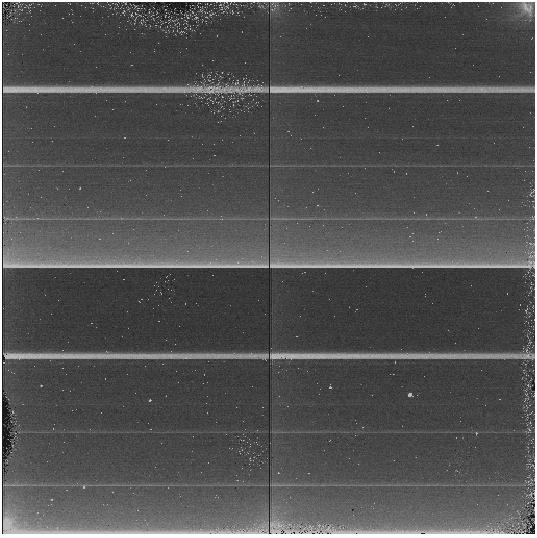

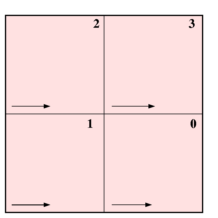
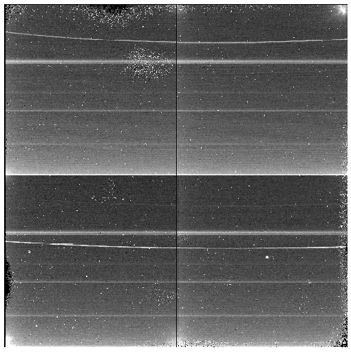
There is a higher brightness in the first few rows in each quadrant where the count level can be more than 3 times the average level in the remaining part of the quadrant. This seems to subtract out well, although the it may take time to stabilize sufficiently that the subtraction is perfect. In dark images of longer integration times there is clear evidence of amplifier glow along the edges. This effect also apparently subtracts out well. There are two dead columns [1,*] and [513,*] along the whole detector, contributing with 0.2 % zero pixels. This is inherent to the controller which has problems with the first column of each quadrant. (Note that since Jan-06 the stored data are flipped in X, and therefore the dead columns are now [1024,*] and [512,*].) Pixels are called bad when they deviate by more than 8 sigma from the mean level. Among the bad pixels we distinguish between hot and cold. The cold pixels include also the zero pixels which show no response at all. The hot pixels may be strongly non-linear. In dark images the amount of hot pixels is 1.4 % (on 42s darks), while in well exposed images the number of hot pixels is < 0.2 %. (Note that this high percentage for the darks is NOT due to the wrap-around effect of very low value pixels in the darks. That effect amounts to only 0.1 % in the cases that have been tested. It is more likely that the hot pixels drown in the higher noise of the exposed dome flats.) The majority of the hot pixels are found close to the edges. The number of hot pixels increases with exposure time. The table below is taken from the Spectroscopic mode commisioning report which has more information also on clusters of hot pixels.
There is a small bad pixel group (mostly hot and non-linear) of about 8 x 9 pixels large, centred at [784,268], or in images taken after Jan-2006 at [240,268]. The majority of the individual bad pixels (hot and cold) are found along edges and corners. There is a region inside the array at [524:674,800:900] which also has an elevated number of individual bad pixels. There are also a few individual bad pixels spread over the whole array. The number of dead pixels was believed to increase with every thermal cycle of the array. This is because of the different thermal expansion properties of the layers of an infrared array, which may cause detachment of the bump bonds upon repeated thermal cycles. However, for the engineering grade array which has undergone a number of thermal cycles during the more than 4 years it has been inside NOTCam, we did not see any increase in the number of zero-level pixels. The apparent coming and going of zero-level pixels was found to be due to a drift in the array causing the reset level to vary. This effect is described under the engineering grade array .
The NOTCam detector quality control is monitoring any change in the
number of bad pixels:
Dark level
Readout noise
ramp-sampling mode Please, check the NOTCam User's Guide for a description of the two different readout modes available with NOTCam.
Gain
The gain is calculated in a representative area in each quadrant.
ramp-sampling mode
Non-linearity
For each readout mode you can check the non-linear behaviour for each
of the four quadrants from the monitoring data: ramp-sampling mode
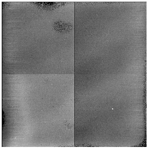
Detector flat field
The detector flat field looks relatively flat and has few disturbing features. The figure above shows the master flat obtained from 10 dome lamp ON images minus 10 dome lamp OFF images for the WF camera and the Ks filter. The standard deviation in small boxes of 20 x 20 pixels is about 2%. The deviation over the whole field is ± 5%. These numbers are the same for the HR camera Ks flat. A worst case diagonal cut through the flat field above is shown here (eps file). The above detector flat field can be compared to the data sheet with the QE image that came with the array (flip in y-direction).
Memory effect (charge persistency)For non-saturated pixels there is memory (or charge persistency) only in the first of the subsequent exposures. The memory effect is negative and the level is 1 % or less. For saturated pixels the memory is more persistent. It is negative in the first subsequent exposure, but positive thereafter. The level is 0.2 % in the 2nd exposure and 0.03 % in the 6th exposure. If you can not avoid saturation, it is recommended to clean the array with a couple of dark 0 commands between each science exposure. The behaviour of the memory effect is illustrated by a series of images shown below.
|
||||||||||||||||||||||||||||||||||||||||||||||||||||||||||||||||||||||||||
|


